
Results Overview
In the following sections, an overview of data available for code assessment/calibration purposes is presented. Data was gathered with the model in three basic configurations: 1) takeoff with full-span flaps, 2) landing with full-span flaps, and 3) landing with part-span flaps. With the degree of flowfield separation and three-dimensionality as a measure, the takeoff configuration is the least challenging computationally while the landing configurations with full-span and part-span flaps are increasingly more difficult.
CFD Validation Data – Lift
Typical lift curves for the takeoff and landing configurations are shown
below. Lift levels are high, relative to current commercial transports
with higher aspect ratio wings and trailing edge flaps that are not full-span.
Maximum lift is reached at angles exceeding 30 degrees, well above stall
angles for conventional transports. These differences do not detract from
the usefulness of the data set for code validation purposes.
Lift curves for landing and takeoff configurations.
CFD Validation Data – Model Pressures
The model is instrumented with static pressure taps on the slats, main element, flap, and body pod. The full-span and part-span models have over 750 pressure taps, aligned in streamwise rows at h=0.17, 0.28, 0.41, 0.50, 0.65, 0.70, 0.85, 0.95, and 0.98. In addition, the flaps have two rows of spanwise pressures on the upper surface, near the pressure minimum and just ahead of the trailing edge.
Pressure coefficients at h=0.28,
0.50, and 0.85 for the full-span landing flaps configuration at Rec=15x106
are shown below. Slat, main, and flap Cp’s are shown for a=10,
20, 26, and 28 (post-stall). As angle of attack is increased, the slat
becomes more heavily loaded, with the outboard sections reaching Cpmin=-13.
Post-stall (a=28 deg),
lift on the main element has dropped dramatically at the mid-span location,
while inboard, the slat and main element remain attached. Peak flap pressures
decrease with increasing angle of attack, due to the displacement effect
of the main element wake , which increases with increasing angle
of attack. The spanwise pressure rows also indicate that the tip’s region
of three-dimensionality extends to roughly h=0.70.
Pressure distributions for the full-span landing
flaps configuration 1. Top to bottom: h=0.85;
h=0.50;
h=0.28; spanwise flap
pressures. M=0.15, Re=15x106.
CFD Validation Data – Wall Pressures
For testing at the 12ft, where wall interference
effects are significant, the signature of the lifting system on the wall
is large. Wind tunnel wall pressures are useful for comparing predicted
and measured wing wall pressure signatures, and for assessing the mass
flow distribution through the three channels formed by the splitter plane
and balance fairings. Throughout the course of testing at the 12ft, pressures
were acquired along 10 streamwise rows of wall pressure taps, as well on
the image plane, along streamwise rows and across the width of the leading
edge. The layout of the wall pressure taps, along with the wall pressure
signature of the landing flaps configuration at
a=10,
20, 26, and 28 degrees is shown in the figure below. The influence extends
more than +/- 3 chords upstream/downstream, and is largest opposite the
model upper surface. Note the large acceleration beneath the splitter plane,
due to the balance fairing.
Layout of wall pressure taps.
Wall pressure signature of the full-span landing flaps configuration
1.
CFD Validation Data – Transition
The sensitivity of high lift system performance to transition locations is well established. Documentation of transition locations was identified early on as a requirement for code validation purposes.
Development of efficient measurement techniques for transition on the slat, main element, and flap upper surfaces proved to be a major challenge. For the initial entry at the 14x22 tunnel (which has no ability to control tunnel total temperature), internal model heating in conjunction with surface temperature measurement using infrared cameras was attempted. The resistive heating elements built into the model lead to highly non-uniform surface temperature distributions. However, because of the large thermal mass of the model and the rapid rise in tunnel total temperature during initial tunnel operation, a significant temperature difference existed between the model surface and tunnel freestream and useful transition data was acquired without any internal heating.
Transition image on main element for full-span landing flaps configuration
1.
For the 12ft entry, a temperature-sensitive paint system was used to acquire surface temperature distributions and infer transition location. This optical thermography technique utilizes the difference in convective heat transfer rates between laminar and turbulent boundary layers. Transition is marked by changes in the surface temperature between the laminar and turbulent regions whenever there is a difference between the model and freestream temperatures.
A temperature difference was introduced by running the tunnel at elevated Mach number (dictated by stress limits) with the tunnel radiator closed. When the model was sufficiently heated (a rise of 15R above equilibrium conditions was desirable), the tunnel Mach number was lowered to the desired condition and the tunnel radiator was opened. Cooling rates of up to 5R/min were obtained.
Temperature sensitive paint (EuTTA in model airplane dope) was applied to the slat and first 25 percent of the main element and flap upper surfaces. A white basecoat was used to enhance surface scattering and increase the luminescent emission of the TSP.
Four 2000 joule photographic strobes were used for illumination; bandpass filters were used on both the strobes and the cameras to reduce stray light. A total of three scientific-graded cooled CCD cameras were used. See Burner et al ("Unified Model Deformation and Flow Transition Measurements", J. Aircraft, Vol 36, No. 5, pp 898-901) for a more details of the system used.
Since TSP brightness varies with temperature, illumination intensity,
and paint thickness, the raw TSP images were corrected by ratioing each
image with a reference image. Above is an example of a ratioed image, taken
at conditions of Pt=1 atm, Rec=3.5 million, alpha = 24 degrees. Note that
only the slat upper surface and forward 25% of the main element and flap
are visible. Transition on the main element is clearly visible as a light-to-dark
region. The spanwise breaks in this light-to-dark region are due the turbulent
wakes behind slat brackets.
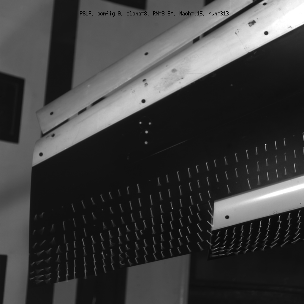
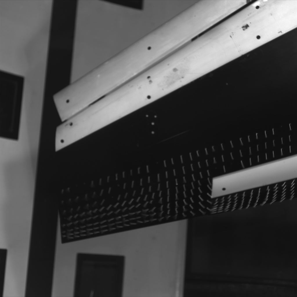
CFD Validation Data – Minituft Images
In order to qualitatively document the stall progression for both the fullspan flap and partspan flap configurations, fluorescent minitufts were applied to the model. These minitufts were 0.0025" in diameter, and were made from a polyester monofilament material. The tufts were attached to the upper surfaces of both flaps, and to the trailing edge region of the main element. The tufts were space approximately 1.5" apart, and were applied from root to tip.
Minituft images of the outboard portion of the part-span landing flaps configuration (0.5 < h < 1.0) are shown in Figure 10a-d. A significant amount of spanwise flow is seen on the flaps at all angles of attack. Flow on the outboard portion of the main element becomes increasing three-dimensional with increasing angle of attack. At a=8 degrees, the influence of the tip is seen over 3 rows of tufts (spanwise variation of 0.2 tip chords). As angle of attack increases, the region of separation grows larger, moving inboard and upstream from the trailing edge. At a=32 degrees (close to maximum lift conditions) the outboard wing is entirely separated, with tufts pointed upstream.
 a=8
deg
a=8
deg
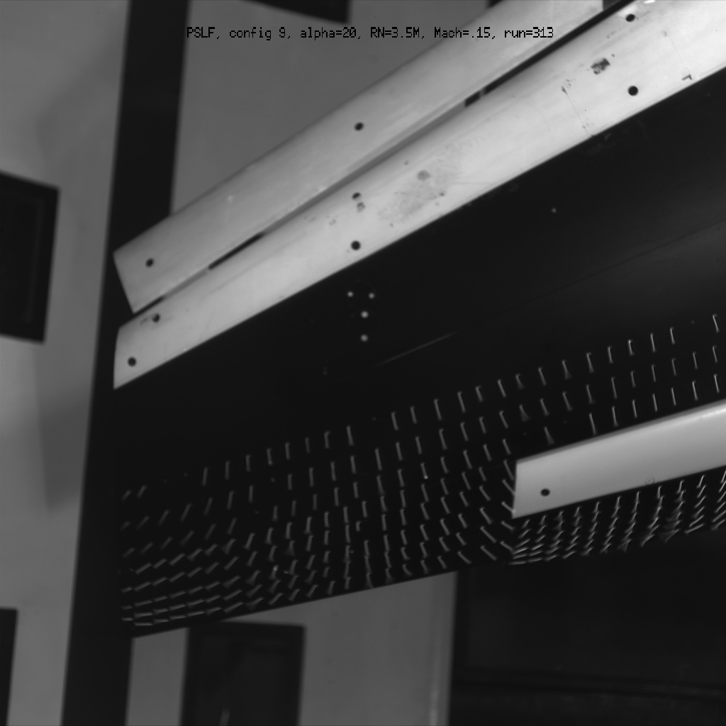 a=20
deg
a=20
deg
 a=28
deg
a=28
deg
 a=32
deg
a=32
deg
Minituft images of part-span flaps landing configuration 9, Rec=3.8x10⁶.
CFD Validation Data – Velocity Profiles
While comparisons between computed and measured forces, moments, and surface pressures is extremely useful, more detailed flow field comparisons may be needed to identify grid generation, solver, and/or turbulence modeling shortcomings. Accurate mean velocity profiles were deemed most critical for code validation purposes, more useful than Reynolds stress measurements that necessarily have larger uncertainties (P. Spalart, private communication). The design, fabrication, and validation of a pressure probe and traverser suitable for a three-dimensional high lift flow field proved to be a major challenge.
Seven-hole probes were purchased from Texas A & M University and calibrated in the Probe Calibration Tunnel of the Flow Physics and Control Branch at NASA-Langley. At the tip, the probes were 0.065 inch in diameter (see figure below).
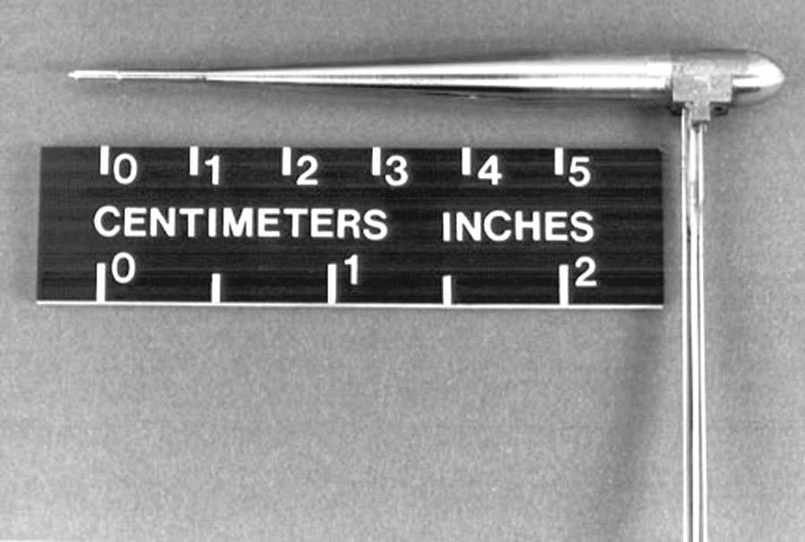
7 hole probe and probe stem.
The probes were calibrated at three total pressures (Pt= 17, 32, 60 psia), from Mach 0.10 to 0.80 in increments of 0.10. The angular range of calibration extended from –20 to +20 degrees in 2 degree increments (in both alpha and beta), and from –20 to –56 degrees and +20 to +56 degrees in 4 degree increments. Approximately 24 test conditions/probe, and 1431 data points/test condition were acquired.
The data reduction procedure divided the probe face into 7 sectors, and data was reduced using recent least-squares and neural-net methods, and checked against least-squares methods developed at NASA-Langley (C. McGinley, private communication).
The overall accuracy for the 7-hole probes has not been estimated at this time. This requires estimating the errors in the pressure measuring system, probe positioning device, and numerical procedure. Calculations of the errors from the calibration procedure at Langley show flow angularity uncertainty to be 0.2-0.4 degrees and velocity magnitude uncertainty to be 0.5% to 1% over the entire Mach-Reynolds number range at angles up to about 20 degrees for the least-squares procedure. Above 20 degrees, the angle uncertainties are 0.3-0.6 deg and velocity uncertainties are 0.5-2%.
A major challenge in the design of a traverser for a complex, three-dimensional flow field is to minimize aerodynamic intrusiveness and relative motion between the probe tip and model. Four legs attached a teardrop-shaped motor fairing to the model lower surface (see figure below). The probe stem protruded through the model, and the probe surveyed the model upper surface at discrete spanwise and streamwise locations. Two fairings shrouded the probe stem on the model lower surface, and were individually yawed to minimize loading on the fairing. The local orientation of the motor fairing (sideslip angle) varied with spanwise location, and was chosen to minimize intrusiveness based on three-dimensional panel code solutions.
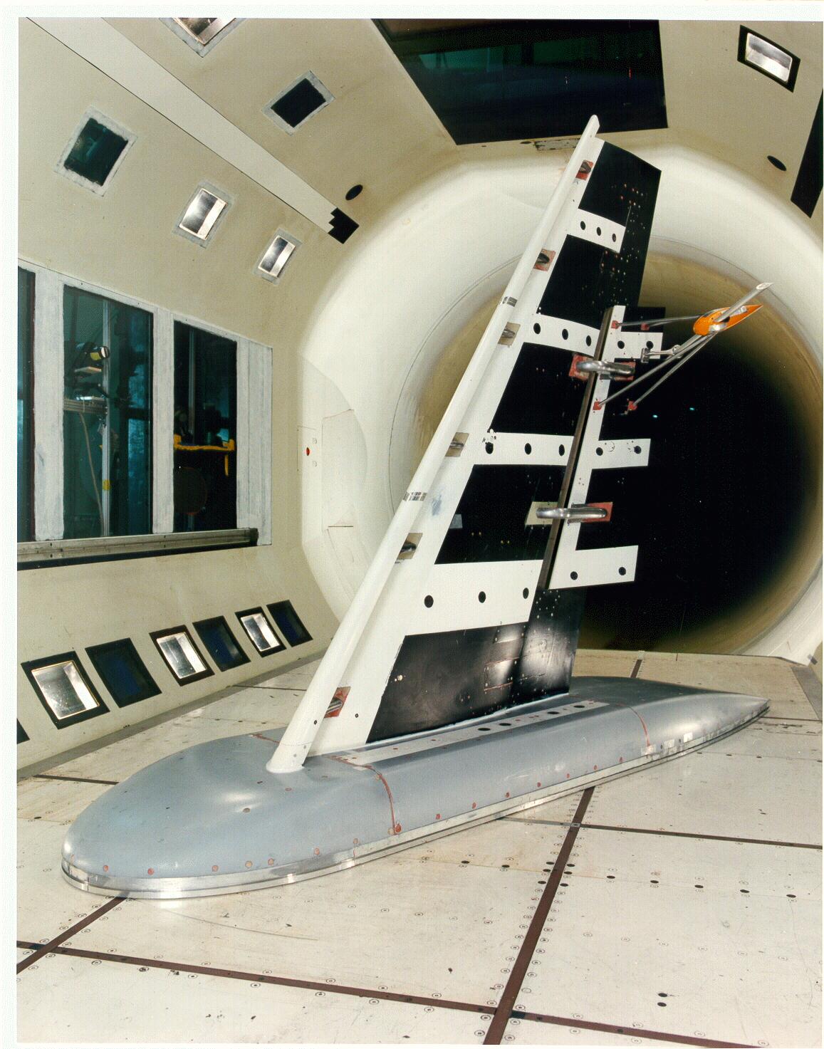
7 hole probe and traverser installed on part-span configuration in ARC12ft. Photo courtesy of NASA.
Comparisons of measured pressure distributions with the traverser on-off allow assessment of the degree of traverser intrusiveness. No significant differences are seen in the main element or flap pressure distributions with the traverser installed at its most aft position on the flap (see figure below).
Traverser intrusiveness with traverser installed at aft flap position,
h=0.85,
a=10
degrees, Rec=4.6x10⁶, full-span landing flaps configuration
1.
Larger Cp differences are seen with with the traverser installed at its most aft position on the main element (see figure below). The local circulation is more strongly affected by the presence of the traverser, due to the alteration of the slot flow approaching the flap. However, boundary layer calculations17 using the measured pressure distributions show that the integrated effect of the pressure perturbations on the boundary layer profile are relatively small, with differences in displacement thickness roughly 4% at the probe tip. These small differences should not alter the data’s usefulness for test-code comparisons of wake spreading and confluency.
Traverser intrusiveness with traverser installed at aft main element
position, h=0.85, a=10
degrees, Rec=4.6x10⁶, full-span landing flaps configuration
1.
For the full-span flap configuration, velocity profile measurements were made at two spanwise locations (h=0.50, 0.85) and at a total of 6 streamwise locations. These locations were chosen from the 11 available (see figure below) as best documenting the streamwise development of the slat, main, and flap boundary layers and wakes in regions with mild (h=0.50) and significant (h=0.85) three-dimensionality.
Available locations of velocity profiles for full-span flaps landing
configuration. X/c relative to stowed configuration.
The streamwise development of the multiple shear layers for the full-span landing flaps configuration 1 is seen in the figure below. Plots of the streamwise velocity component U/U¥ show the streamwise development of the shear layers. At low angles of attack (a=10 degrees), the slat is lightly loaded and the slat wake that is clearly visible at x/c=0.10 has disappeared near the trailing edge of the main element (x/c=0.72). At higher alpha, the slat wake is still evident at x/c=0.72 and has become confluent with the main element boundary layer. On the flap, near Cpmin (x/c=0.85), the wake size and velocity deficit from merged slat/main element wakes increase with increasing alpha. Note that the flap boundary layer is thin at this forward location and was not measured. At the trailing edge of the flap (x/c=1.05), the main element wake grows dramatically as angle of attack increases from 10 to 20 degrees. At a=24 degrees, the main element wake has reversed and an off-body separation is present above the flap.
 a) a=10,
x/c=0.10
a) a=10,
x/c=0.10 b) x/c=0.72
 c) x/c=0.85
 d)
x/c=1.05
d)
x/c=1.05
Velocity profiles on the full-span landing flaps configuration 1, Rec=8.8x10⁶. a) x/c=0.10; b) x/c=0.72; c) x/c=0.85; d) x/c=1.05.
return to Data Archive home page
Page Curator and NASA Official Responsible for Content
Judith A. Hannon
Last Updated
August 5, 2011