DATA SUBMITTAL FORMS & POSTPROCESSING INFO
5th
AIAA CFD High Lift Prediction Workshop
Much of the data required for HLPW-5 is the same as for HLPW-4. However, one notable exception is pressure and
skin friction coefficient extraction location.
Details are provided below.
Return to: High Lift Prediction Workshop Home Page
Data Submittal Forms
The Tecplot-readable Data Submittal Forms are provided in the following tarred gzipped directories:
Also, please submit a 1-page-only (Powerpoint or PDF) summary of your method:
DETAILED INSTRUCTIONS FOR PREPARING DATA SUBMITTAL FORMS
- Data should be submitted in a logically-named directory that includes your PID (in place of the "XXX"), your last name, code, model, and any
other important identifying information. Download the above tarred gzipped directory, unzip and untar it, then rename it. Also rename
all subdirectories below it.
If you are submitting only one set of data for a given test case, then the subdirectory name should end with BESTPRACTICE. For example,
L. Wang might have the subdirectory names:
- "W-005_Case1_Wang_FUN3D_WMLESVreman_BESTPRACTICE" for Case 1
- "W-005_Case2.1_Wang_FUN3D_WMLESVreman_BESTPRACTICE" for Case 2.1
- "W-005_Case2.2_Wang_FUN3D_WMLESVreman_BESTPRACTICE" for Case 2.2
- "W-005_Case2.3_Wang_FUN3D_WMLESVreman_BESTPRACTICE" for Case 2.3
- "W-005_Case2.4_Wang_FUN3D_WMLESVreman_BESTPRACTICE" for Case 2.4
- "W-005_Case3.1_Wang_FUN3D_WMLESVreman_BESTPRACTICE" for Case 3.1
- "W-005_Case3.2_Wang_FUN3D_WMLESVreman_BESTPRACTICE" for Case 3.2
- "W-005_Case3.3_Wang_FUN3D_WMLESVreman_BESTPRACTICE" for Case 3.3
- "W-005_Case3.4_Wang_FUN3D_WMLESVreman_BESTPRACTICE" for Case 3.4
where W-005 is L. Wang's team's assigned PID.
A typical submission will consist of one subdirectory of data per case.
Submitting results for only a subset of the cases is allowed.
Partial results (e.g., results for only a few AoAs out of the total number requested) are also allowed...
simply fill in what you have.
All results in a subdirectory should use the same methodology (same turbulence model, numerical method, etc.).
- If you are part of a team, then you should use just one PID and choose just one member's last name in the
title of your directory/subdirectories.
- All filenames should be renamed with your PID, e.g., G-011, R-048, A-002, H-013,
L-025, W-047, W-047.1, W-047.2. For example, XXX_case1_gridconvergence_FM.dat should be changed to R-048_case1_gridconvergence_FM.dat
for participant R-048.
- Inside each data submittal file, replace ALL occurrences of XXX with your assigned PID, especially in all "ZONE T" lines.
Other than the XXX, please do not change the names of any zones inside the files.
- Some data files include DATASETAUXDATA lines. Please fill out as appropriate, being sure to keep the quotes (" ").
- Make sure the number of columns of data you provide in each file EXACTLY MATCHES the number of variables in the variable list!!!
- Please include your surface streamline pictures under the sub-subdirectory XXX_caseX_SurfaceFlowVisualizations. The
preference is that you submit png format, if possible. Use the recommended "CFD views", and
name them
- XXX_aoaYYY_stream_cfdview_01.png
- XXX_aoaYYY_stream_cfdview_02.png
- XXX_aoaYYY_stream_cfdview_03.png
- etc.
corresponding to the views shown on https://hiliftpw.larc.nasa.gov/Workshop5/DataForm.html. Change the XXX in
the filename to your PID and the YYY in the filename to the angle of attack; for example:
"H-013_aoa11_stream_cfdview_01.png".
Include additional descriptive information to
the name if needed.
- Please include your surface Cf contour pictures in the same sub-subdirectory
(XXX_caseX_SurfaceFlowVisualizations). Use the recommended "CFD views" for Cf, and
name them
- XXX_aoaYYY_cf_cfdview_01.png
- XXX_aoaYYY_cf_cfdview_02.png
- XXX_aoaYYY_cf_cfdview_03.png
- etc.
- If supplying them, please include your off-body vorticity plots under the sub-subdirectory XXX_caseX_OffBodyVorticity.
Use the recommended "CFD views", and name them
- XXX_aoaYYY_vort_cfdview_11.png
- XXX_aoaYYY_vort_cfdview_12.png
- XXX_aoaYYY_vort_cfdview_13.png
- etc.
- XXX_aoaYYY_vort_cfdview_11+grid.png
- XXX_aoaYYY_vort_cfdview_12+grid.png
- XXX_aoaYYY_vort_cfdview_13+grid.png
- etc.
corresponding to the views shown on https://hiliftpw.larc.nasa.gov/Workshop5/DataForm.html. Change the XXX in
the filename to your PID and the YYY in the filename to the angle of attack; for example:
"H-013_aoa11_vort_cfdview_11.png".
Include additional descriptive information to
the name if needed.
- Test Cases 2 and 3 also include an optional sub-directory named XXX_caseX_OtherGridsInThisFamily_Results_and_Pics,
where you can provide detailed results from grids other than the "nominal" grid. Instructions are provided
in a README file inside this sub-directory.
- Be sure to fill out the file XXX_participant_info.dat located within each subdirectory. This identifies you and
your method, among other things, for that subdirectory.
Note that some information gets repeated, but it's best for each subdirectory to have complete information.
- Each subdirectory should include ALL the test case data files that
you choose to participate in.
Before tarring or zipping up your directory or subdirectories, remove any files that you are not using. For example, if you
are not providing any velocity data, then remove all files "*_velocity.dat" from the subdirectories.
- If you need to update your results prior to the deadline, then re-send the entire directory or altered subdirectories again.
Assume that we will throw away your old version and start reading everything from the new one.
Edit the file XXX_participant_info.dat in the altered subdirector(ies) and provide: (1) the
date of the latest submission and (2) a list of things changed, added, or subtracted since the last
submission.
- If you are submitting multiple sets of data (for example, different grid types, different turbulence models, different
methodologies, etc.) then
EACH DISTINCT SUBMISSION SHOULD HAVE ITS OWN DIRECTORY OF DATA, and each of your datasets
should have an appended number ".1", ".2", ".3", etc. added to the PID in order to distinguish between them.
For example, if your PID is A-132, you would use A-132.1, A-132.2, A-132.3,
etc. for multiple distinct types of submission variants.
Include the phrase "BESTPRACTICE" only at the end of the subdirectory that you consider to be your "best practice" result.
For example, the A-132 team might want to submit 5 subdirectories of distinctly different
results for Case 1, one of which they consider to be their "best practice" set:
- A-132.1_Case1_Smith_BCFD_SA_limiter_central2ndorder_BESTPRACTICE
- A-132.2_Case1_Smith_BCFD_SA_limiter_upwind2ndorder
- A-132.3_Case1_Smith_BCFD_SA_limiter_upwind3rdorder
- A-132.4_Case1_Smith_BCFD_SST_timeaccurate_central2ndorder
- A-132.5_Case1_Smith_BCFD_SA_nolimiter_central2ndorder
The corresponding PID (A-132.1, A-132.2, A-132.3, etc.) should be used within each respective subdirectory.
- If possible, please test all of your files with Tecplot, to make sure that the Tecplot software can successfully
read them without error, prior to submitting.
- Submit your tarred or zipped subdirectory (for a particular case) or full directory (for all cases)
to Li Wang.
If the file is too large to email, then contact
Li Wang to arrange for file transfer in another way.
Please do not re-organize the data structure provided in
the datafile directory. Your directory(ies) of results should maintain the original look and organization of the above
downloadable gzipped tar file.
Postprocessing: Mean Surface Pressures and Skin Friction Extraction
The surface data are to be extracted along several stations that vary slightly for each of the three test cases.
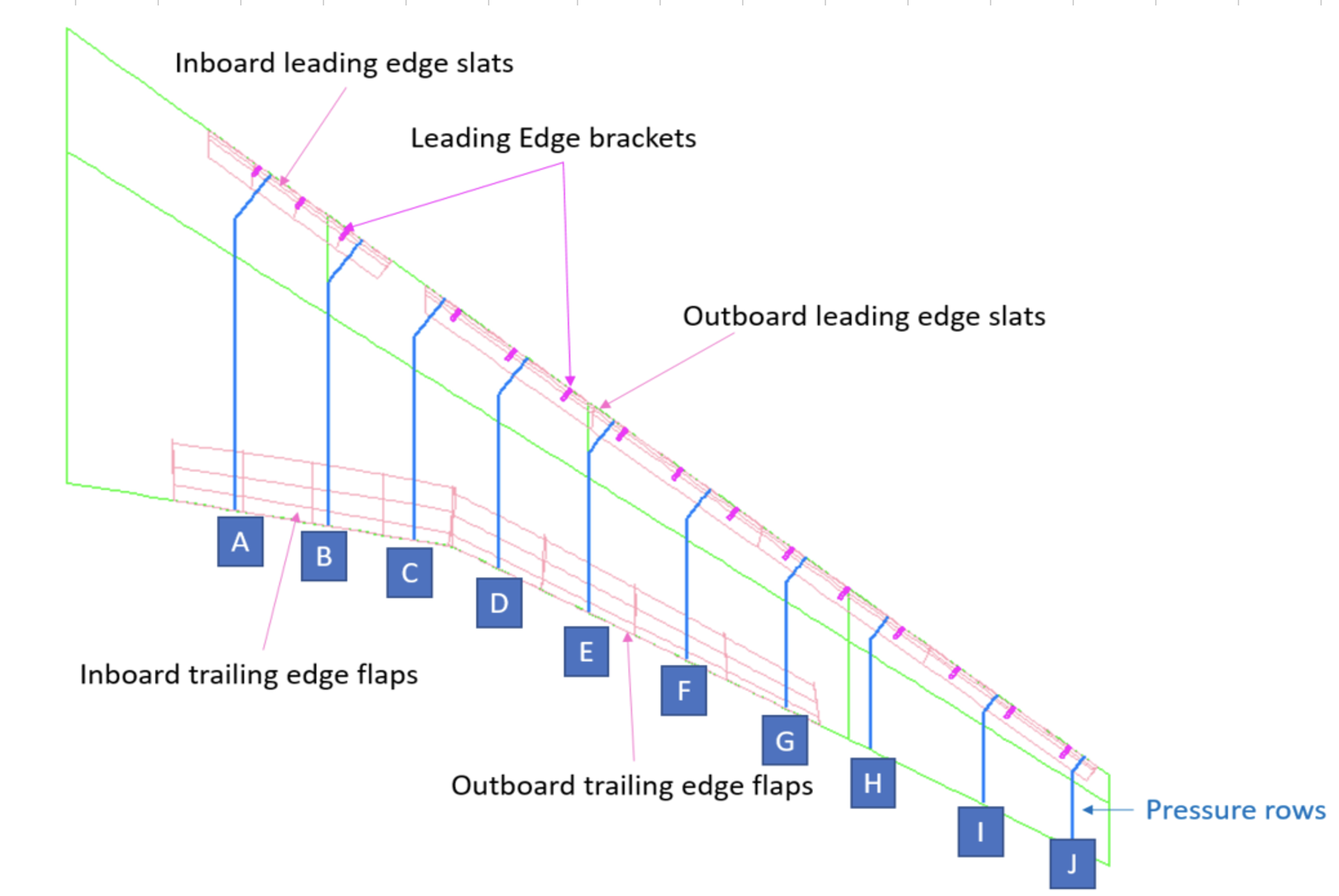
The following figure shows the basic layout with the slat and flap in their stowed positions. On the wing,
there are 10 stations, or "rows" (A through J).
Each pressure tap row is defined by 2 different planes: one approximately normal to the wing leading edge (near the
leading edge) and one approximately along y=constant behind that.
Note that, when deployed, the pressure tap rows are not aligned on all 3 elements (they are aligned only when stowed).
And the deployed flaps only have 7 rows.

The configuration is defined in the +Y plane, in full-scale inches. The following file defines equations
(Ax + By + Cz = D) for the planar cuts on the wing that approximately intersect the
pressure taps for the span stations on the main wing, slat, and flap when in deployed position:
Pressure_Belt_Planes_bodycoordsonly.xlsx or
Pressure_Belt_Planes_bodycoordsonly.pdf.
Participants are also asked to extract surface data along 2 lines on the fuselage, as defined in
the following:
Pressure_Belt_Planes_fuselage.pdf.
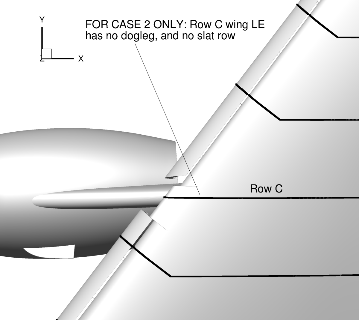
Note that Test Case 1 is slightly different because it only has a main wing (no slat or flap). Test Case 2 is slightly different because
Row C on the wing does not include a dog leg, and
some of its sub-cases do not include slat and/or flap. Test Case 2 also includes an empennage; participants are asked to
extract data on the horizontal tail as defined in the following:
Pressure_Belt_Planes_horiztail.pdf.
For those participants with access to Tecplot, macro files are provided here that can be used to help extract data on the surface
of the full-scale configurations (inches) along all of the
requested pressure tap planes:
- Test Case 1:
- Test Case 2:
- Test Case 3:
In the wing cutters, the locations of the "dog leg" turns in each row were approximated at:
- Row A: x=1126.61 inches
- Row B: x=1199.86 inches
- Row C: x=1266.16 inches
- Row D: x=1332.41 inches
- Row E: x=1402.17 inches
- Row F: x=1478.90 inches
- Row G: x=1555.64 inches
- Row H: x=1621.91 inches
- Row I: x=1709.11 inches
- Row J: x=1778.87 inches
The wing cutters will produce 2 zones for each line of pressures on the wing:
e.g., "Row A wing LE" and "Row A wing". These can be plotted together (Cp as a function of x).
Note that Row C for Case 2 does not include the dog leg and there is no specific slat row. However, to keep the same number of extracted zones
over the slat/wing/flap collection (to make plotting easier), the Row C wing LE part is still extracted separately, and an UNUSED Row C slat part is still included
in the cutter (it should simply be avoided when plotting Case 2 results).

For the different configurations, use only the cutters that apply for the case.
This involves performing the following steps:
- SLAT: For any case with slat present, turn off all but the slat element(s) and use the appropriate slat_cutter macro to extract slices on the slat;
this will produce one zone for each slat row
- WING: For all cases, turn off all but the wing element(s) and use the appropriate wing_cutter macro to extract slices on the wing;
this will produce two zones for each wing row
- FLAP: For any case with flap present, turn off all but the flap element(s) and use the appropriate flap_cutter macro to extract slices on the flap;
this will produce one zone for each flap row
- FUSELAGE: For all cases, turn off all but the fuselage element(s) and use the appropriate fuselage_cutter macro to extract slices on the fuselage;
this will produce one zone for each fuselage row
- HORIZONTAL TAIL: For Case 2 only, turn off all but the horizontal tail element(s) and use the horiztail_cutter macro to extract slices on the horizontal tail;
this will produce one zone for each horizontal tail row
Some editing of the macros may be required... see instructions inside the file.
Note that these macros define each cutting plane by specifying 3 sets of X,Y,Z coordinates that lie in the plane, as defined by the equations in
the above Pressure_Belt_Planes_... files.
Also, be aware that the Tecplot extraction will include ANY active surface cut by a specified plane, even if unintended.
(For the purposes of the workshop, this is acceptable.)
The macro files can be edited. For example, if you know for your grid that you want to
turn off zones 1 and 5 when extracting on a particular element, it can be done with:
$!ActiveFieldMaps -= [1]
$!ActiveFieldMaps -= [5]
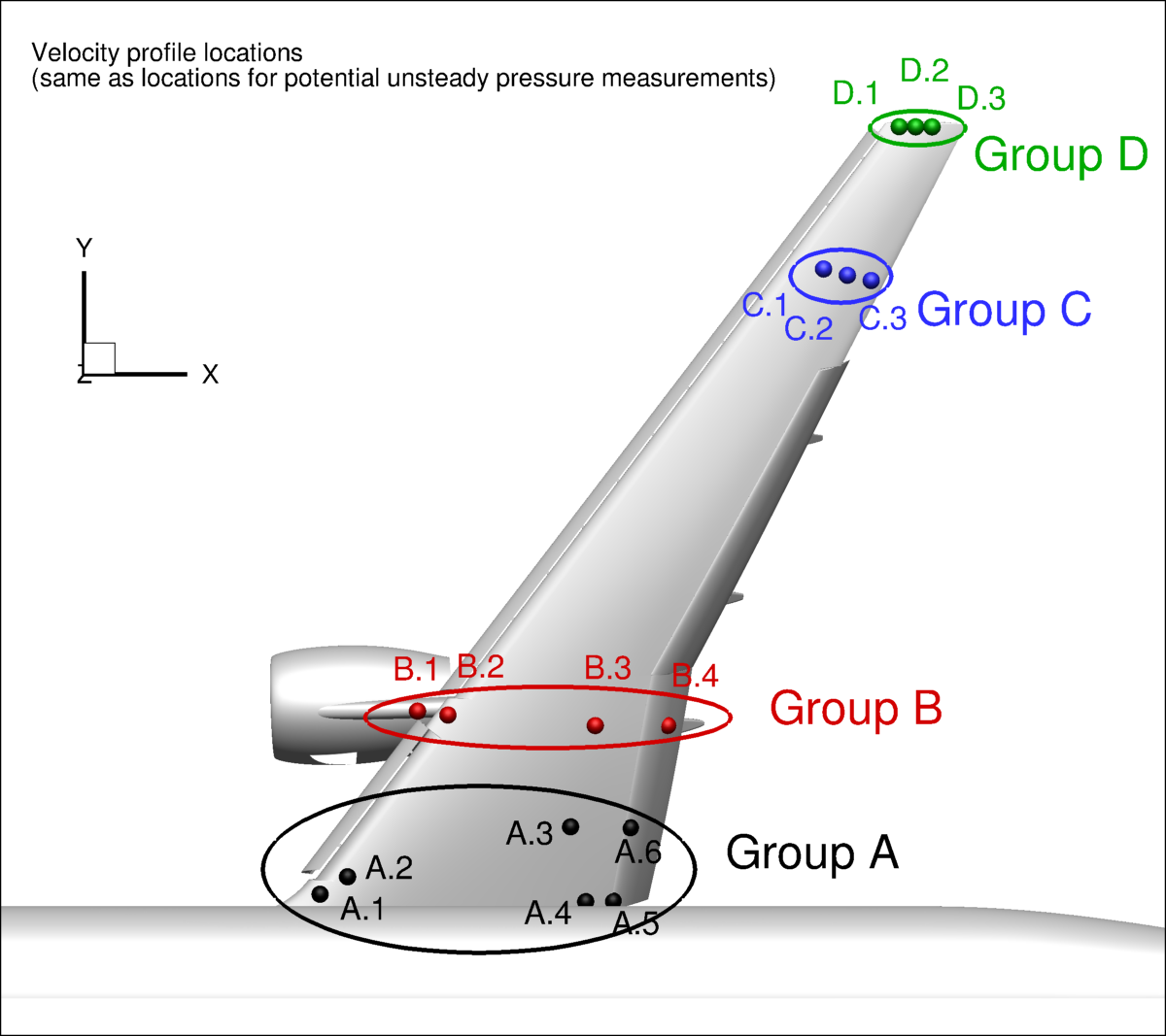
Postprocessing: Velocity Profiles and Unsteady Surface Pressures at Specific Locations on the Wing
Velocity profiles and unsteady surface pressures are being requested at the same locations over the wing.
The locations are identified in the figure below. These correspond to locations where unsteady pressure measurements
may be made in future wind tunnel tests (on the model upper surface). For velocity, profiles should be
extracted along z at the given specific x and y locations (provide enough z-height to include at least all
the boundary layer and any upstream-element wakes... giving too much will not hurt).
The z-direction is with respect to the aircraft reference frame as given in the original CAD files; i.e., the location of
the lines of data along z should be identical regardless of the angle of attack.
For unsteady pressures (relevant only for time-accurate
simulations), data should be extracted on the wing upper surface.

The locations are listed in the files:
kulite_locations_hlpw5.dat.
IMPORTANT: for some of the test cases (including the Case 1 wing-body and some of the Case 2 configuration build-up),
points B.1 and B.4 do not lie on a solid surface. Nonetheless, to ease the plotting process for all workshop data,
these lines should still be included in the submitted data.
Postprocessing: Upper Surface Streamlines and Skin Friction Coefficient (Cf) Contours
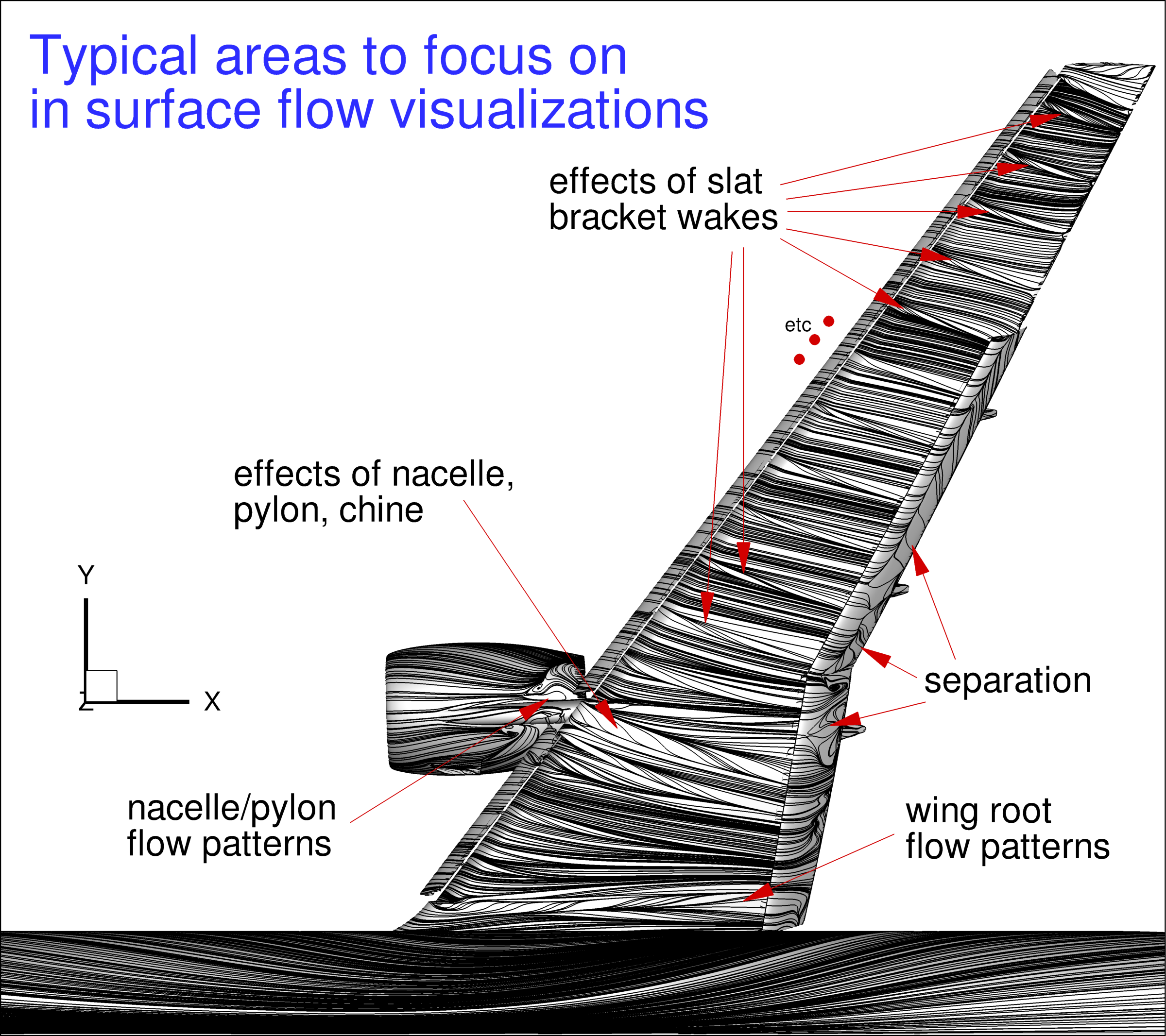
A major set of desired inputs from the CFD are computed surface streamlines (particularly on the CRM-HL configuration's
upper surface), for comparison with surface oil
flow photos. This is particularly important for ascertaining the agreement/disagreement with
regions of separation and other flow features of interest from the experiment.
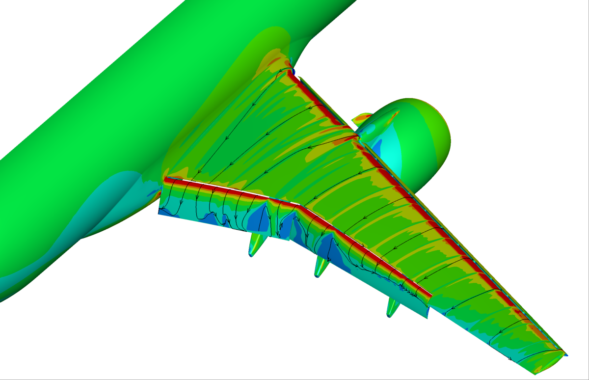
Below is an example surface streamline plot, showing typical areas of interest for HLPW-4.
There are many methods available for obtaining postprocessed surface streamline patterns; at this time, participants
are encouraged to make use of the best tools at their disposal.
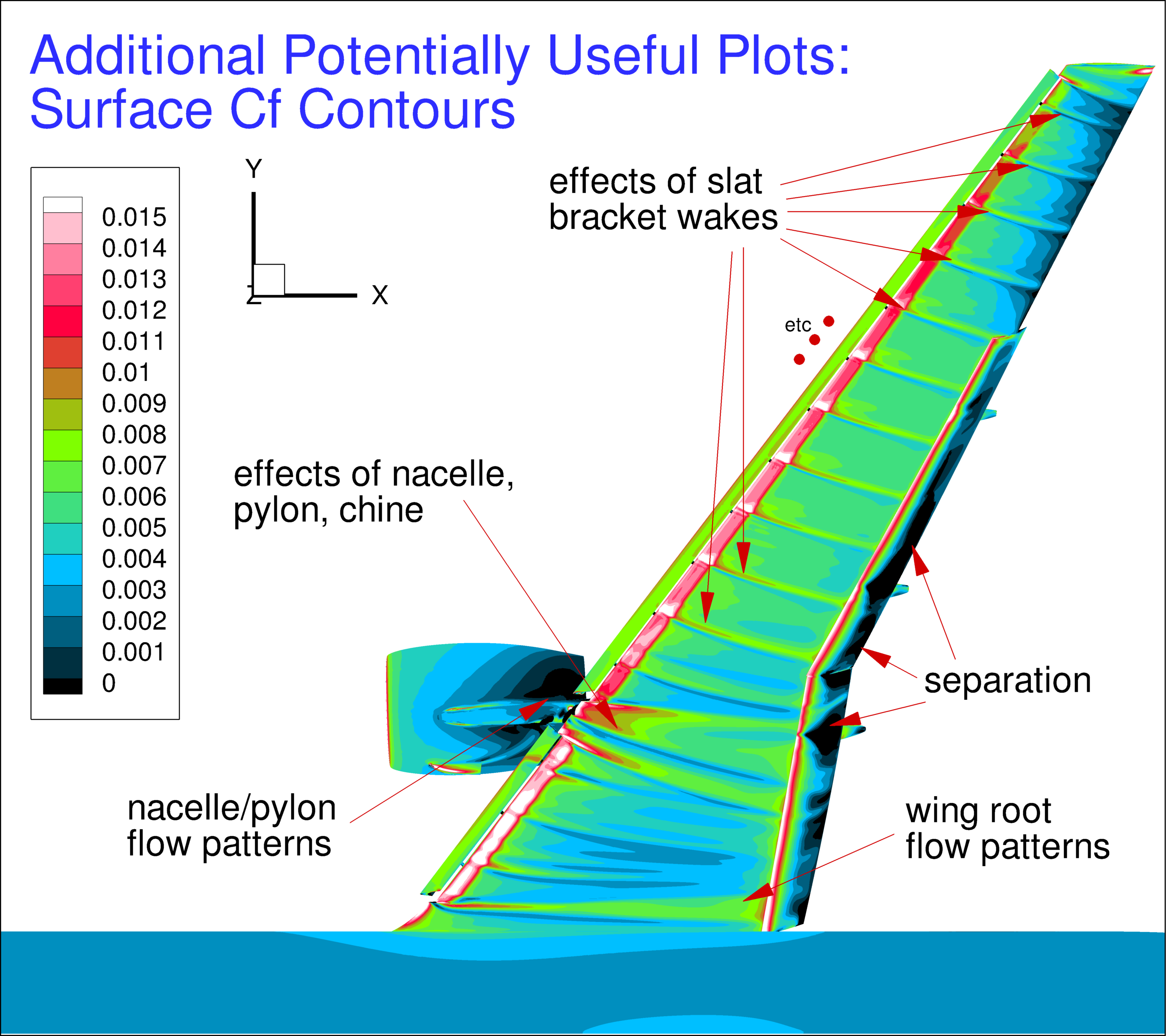
Contours of surface skin friction coefficient are also very useful to plot (see second figure immediately below).
We are requesting plots of total skin friction (tau_w/freestream dynamic pressure), not plots of its x-component.
Note that the definition of tau_w is standard: see, e.g.,
Wall Shear Stress Definition, with the
derivative of the flow velocity parallel to the wall used in the equation.
If your method is unsteady, then mean streamlines and skin friction contours should be plotted.
In the second figure, the Tecplot color map is provided as
cfmap_tecplot.map. It is given by:
| LEVEL
|
R
|
G
|
B
|
| 0.00
|
0
|
0
|
0
|
| 0.25
|
0
|
191
|
255
|
| 0.50
|
127
|
255
|
0
|
| 0.75
|
255
|
0
|
64
|
| 1.00
|
255
|
255
|
255
|
and the recommended range (shown in the figure) is 0 to 0.015, step 0.001 (banded). In the Cf plot, the "lighting" has been turned off;
this reduces the 3-dimensional appearance of the objects, but it improves the interpretability of the colors.
If everyone removes lighting and follows the color scheme and range detailed here, then the resulting CFD
plots should be reasonably easy to compare directly with one another.
The Tecplot layout files for the above two pictures are provided here (minus the arrows and extra words):
XXX_stream_cfdview_01.lay and
XXX_cf_cfdview_01.lay.
However, note that these files are most likely NOT directly applicable to most participants' surface grid or surface data; therefore
they should be used for guidance only (also, different surface streamline seeding may yield better visualizations; this is
an example only).
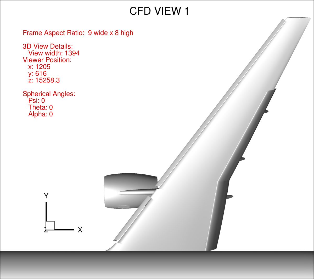
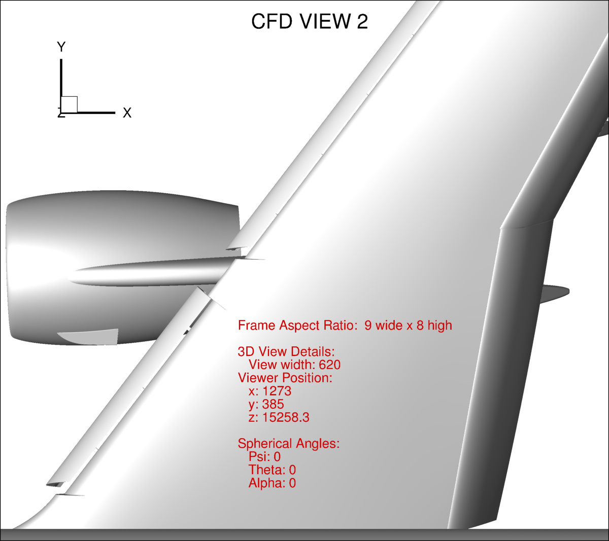
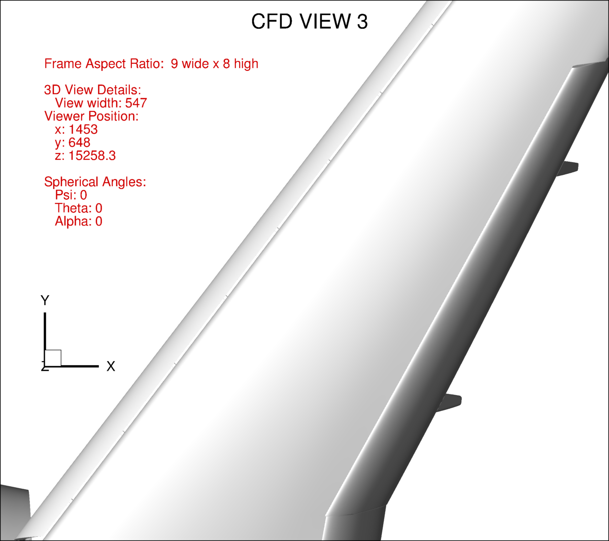
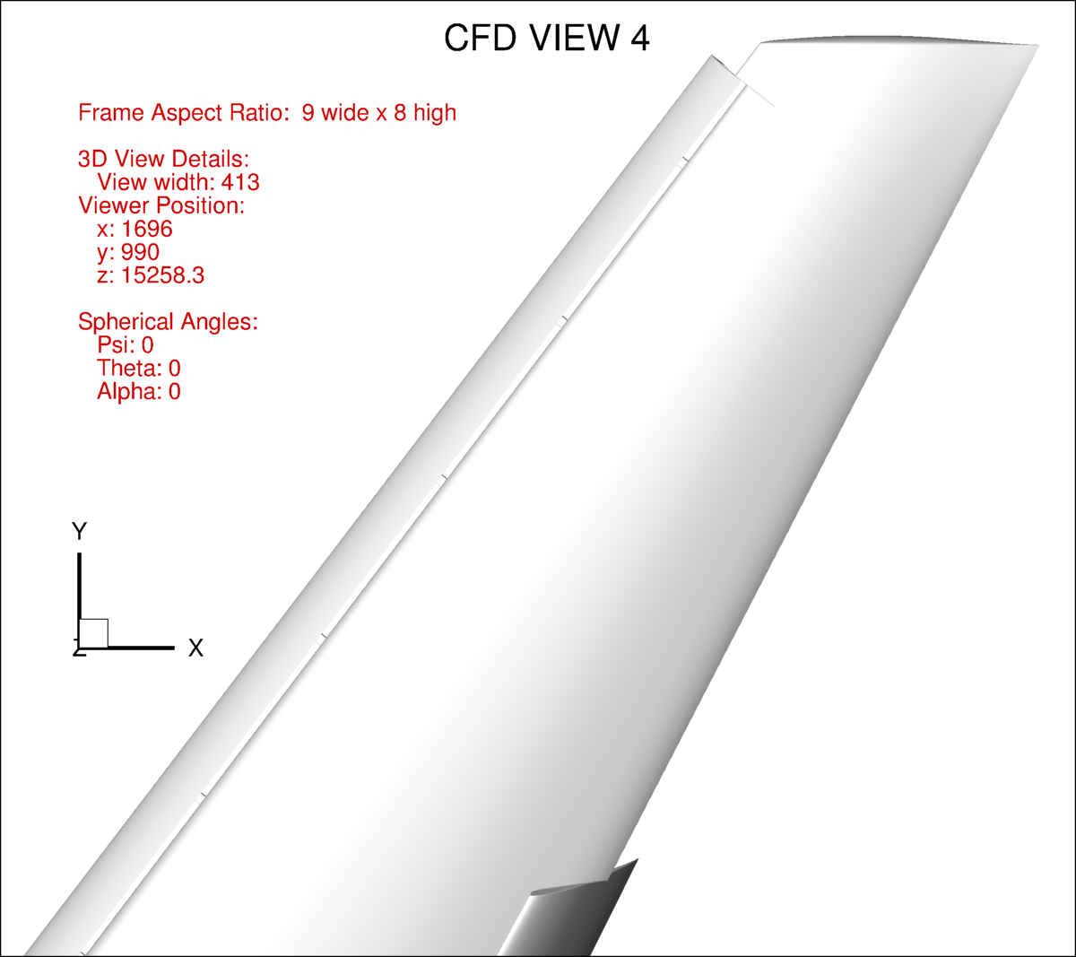
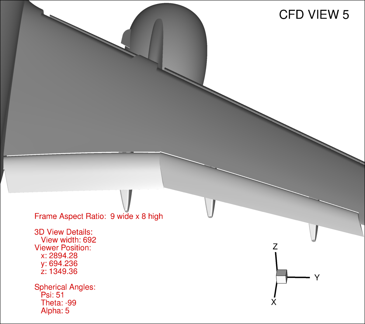
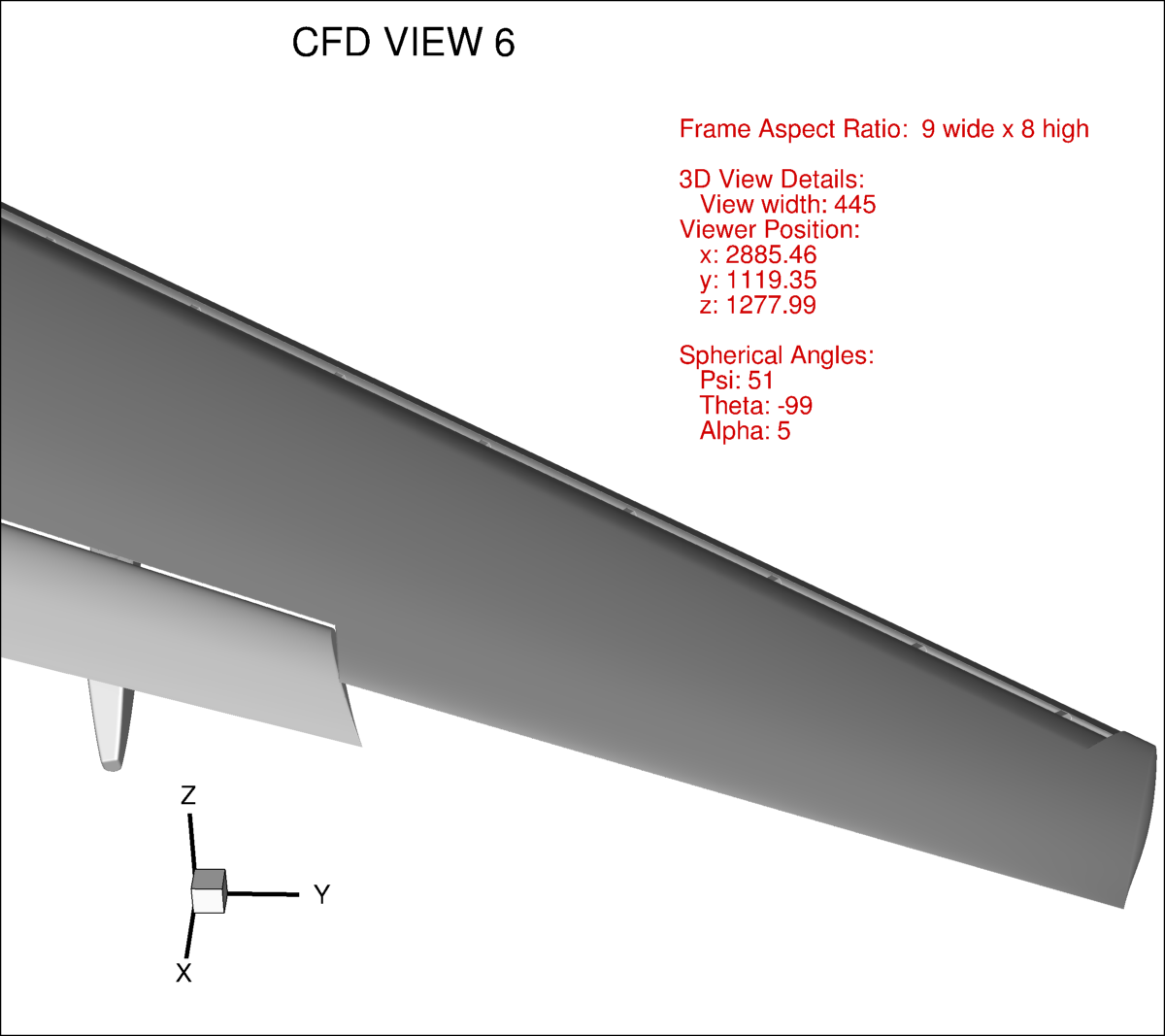
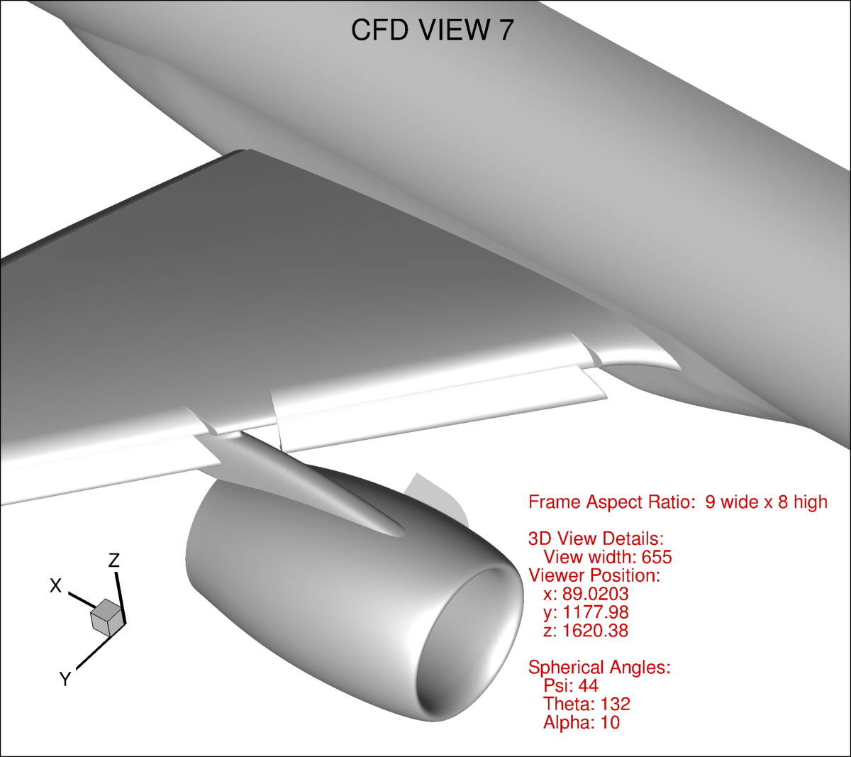
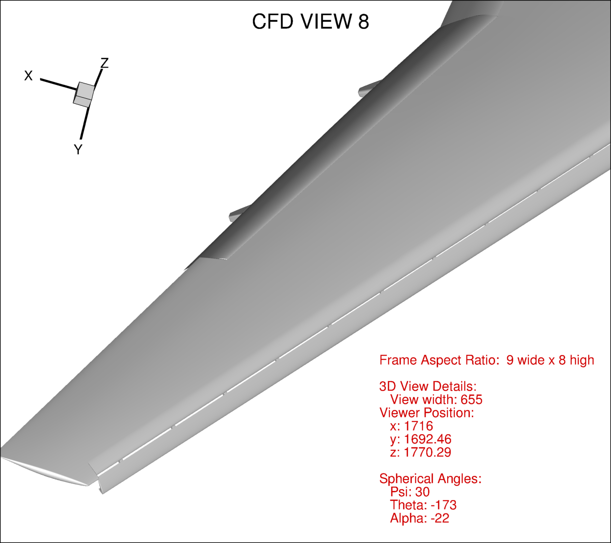
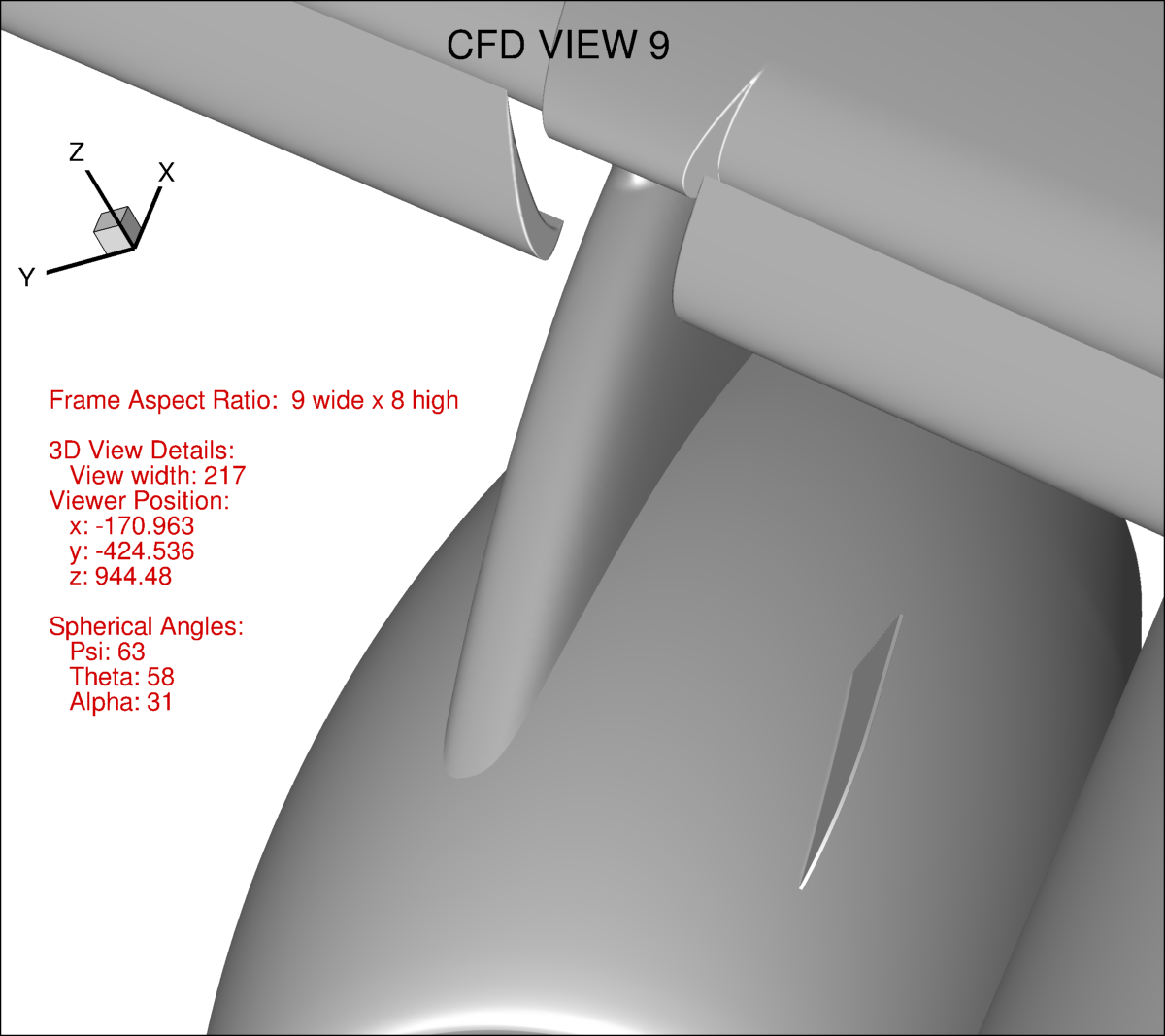
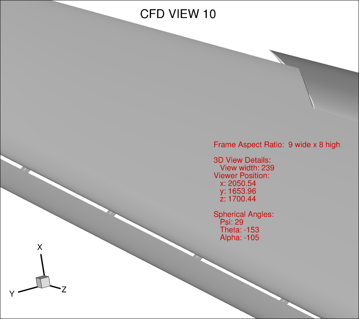
For direct CFD comparisons with other CFD, some recommended views (including Tecplot nomenclature for orientation) are shown below,
where the configuration is in full-scale inches.
In Tecplot, the "use perspective" feature is not turned on for any views.
The CFD views 1-4 are the simplest, taken looking directly down on the configuration (psi=theta=alpha=0);
they should be relatively easy to approximately match, even if only trying to recreate the views using visual cues.
The best views for direct comparisons with wind tunnel oil flow photos are not known, and are currently up to each participant.
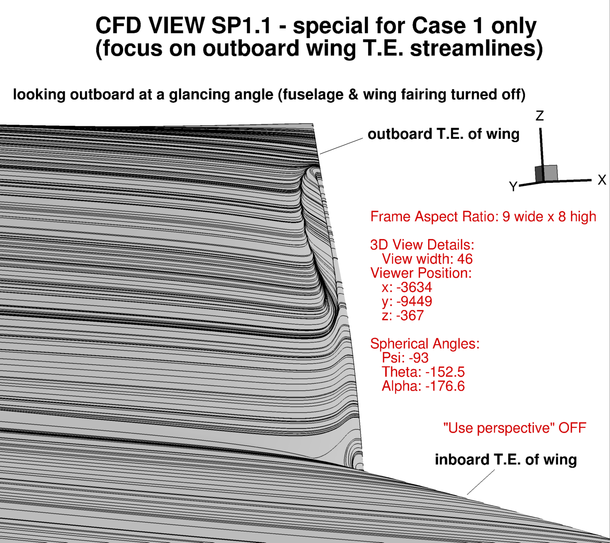
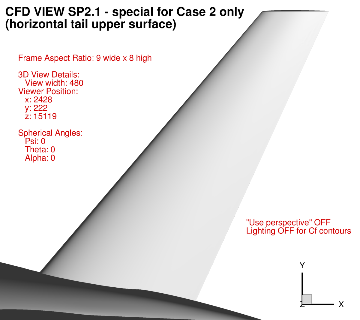
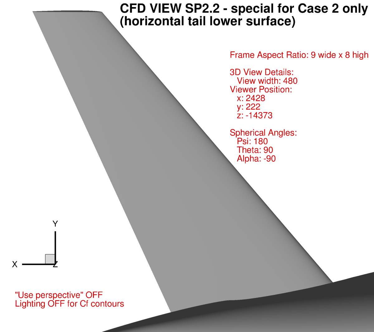
NOTE: Ten views are shown for the high-lift configuration.
Please provide as many as you are able. Priority views are 1 through 5. However, a
special view SP1.1 has been added specifically for Case 1, to help highlight the trailing edge separation on the outboard wing,
and special views SP2.1 and SP2.2 have been added for Case 2, focusing on the horizontal tail.


The Tecplot layout files for the above ten pictures are provided here:
XXX_cfdview_01.lay,
XXX_cfdview_02.lay,
XXX_cfdview_03.lay,
XXX_cfdview_04.lay,
XXX_cfdview_05.lay,
XXX_cfdview_06.lay,
XXX_cfdview_07.lay,
XXX_cfdview_08.lay,
XXX_cfdview_09.lay,
XXX_cfdview_10.lay,
XXX_cfdview_SP1.1_case1special.lay,
XXX_cfdview_SP2.1_case2tail_upperspecial.lay,
XXX_cfdview_SP2.2_case2tail_lowerspecial.lay.
However, note that these files are most likely NOT directly applicable to most participants' surface grid or surface data; therefore
they should be used for guidance only.
Postprocessing: Off-Body Vorticity Contours
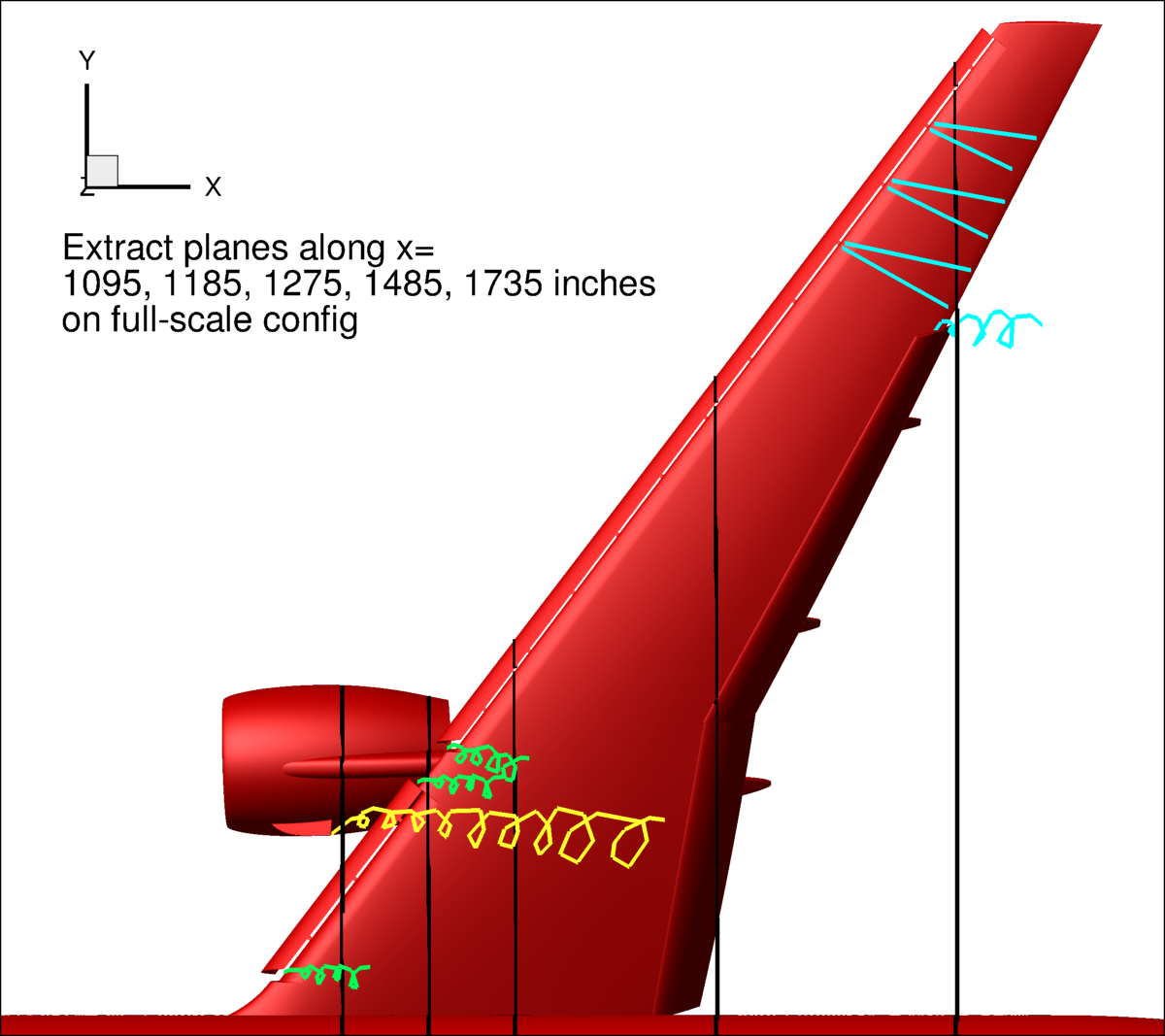
Vortices shed from upstream elements play a major role in the CRM-HL flowfield. We are asking participants to
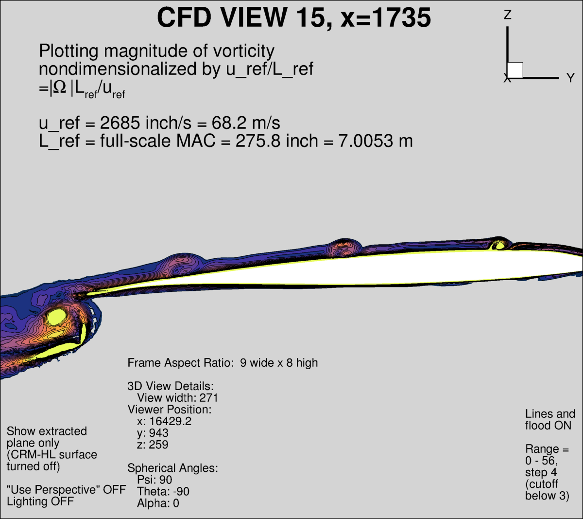
plot nondimensional magnitude of vorticity contours extracted at the 5 planes shown here, for the purpose of making
direct comparisons between different CFD codes and methods:
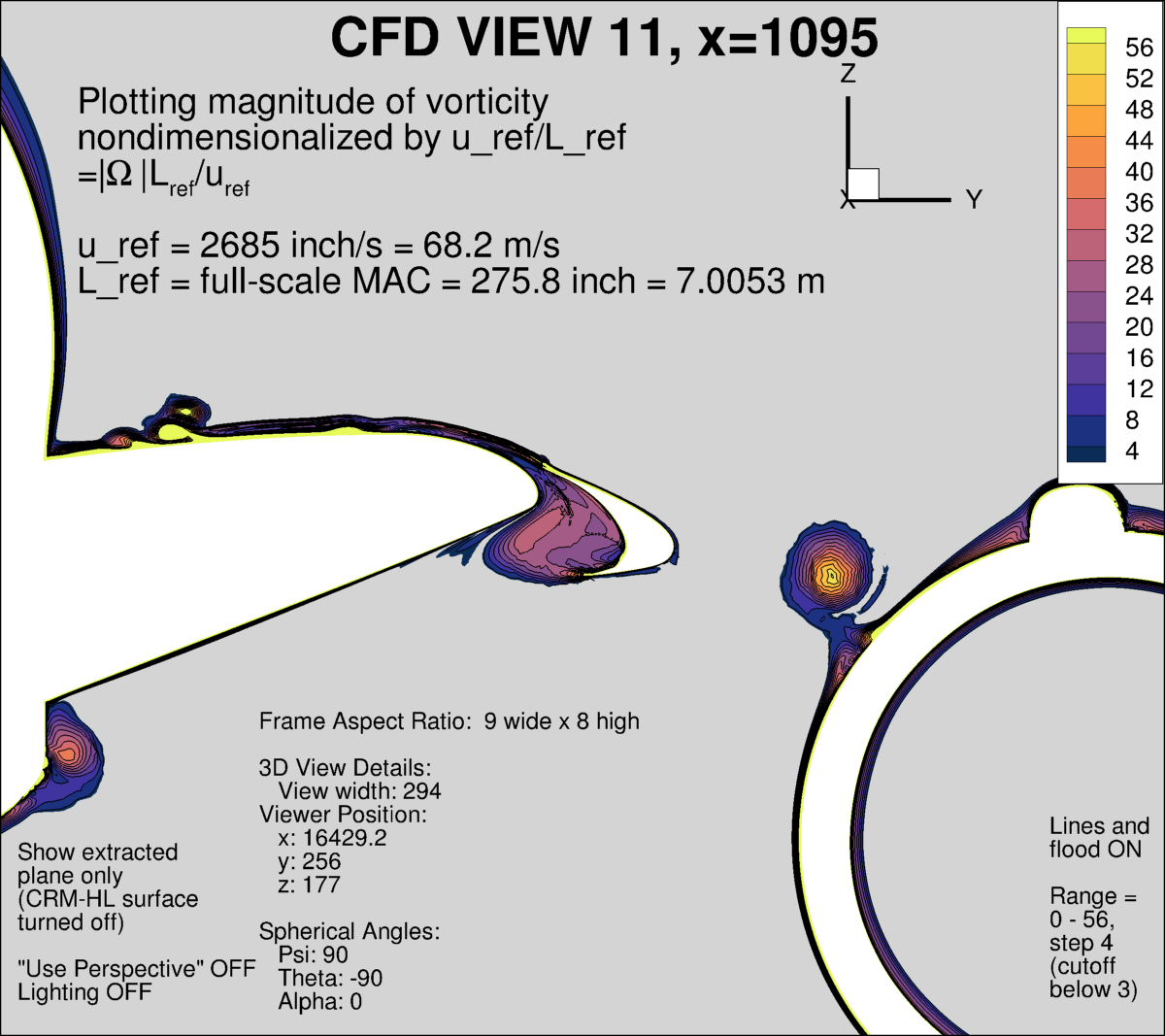
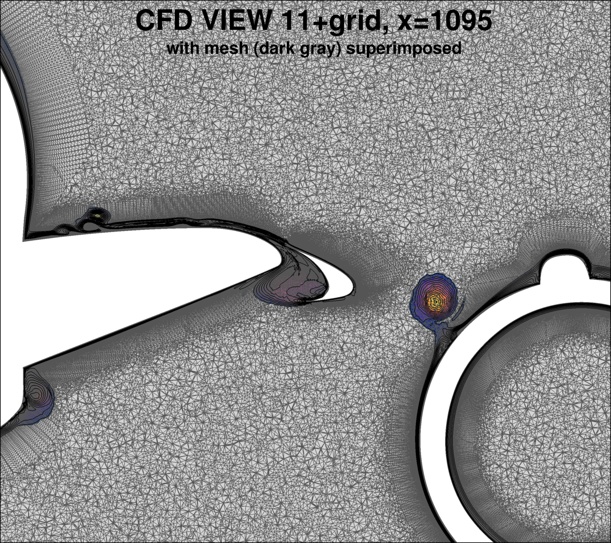
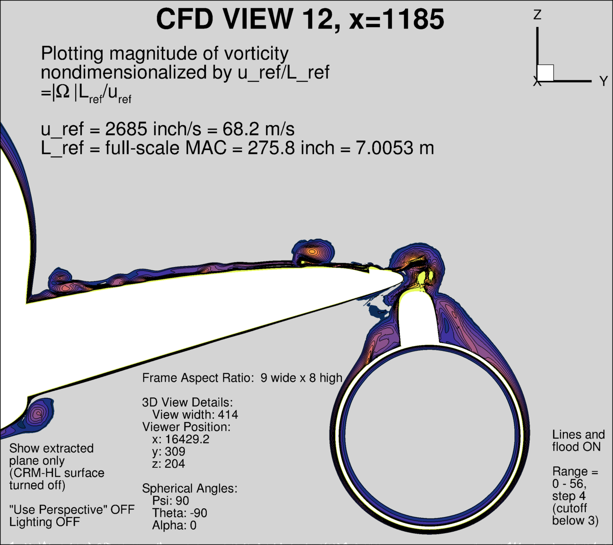
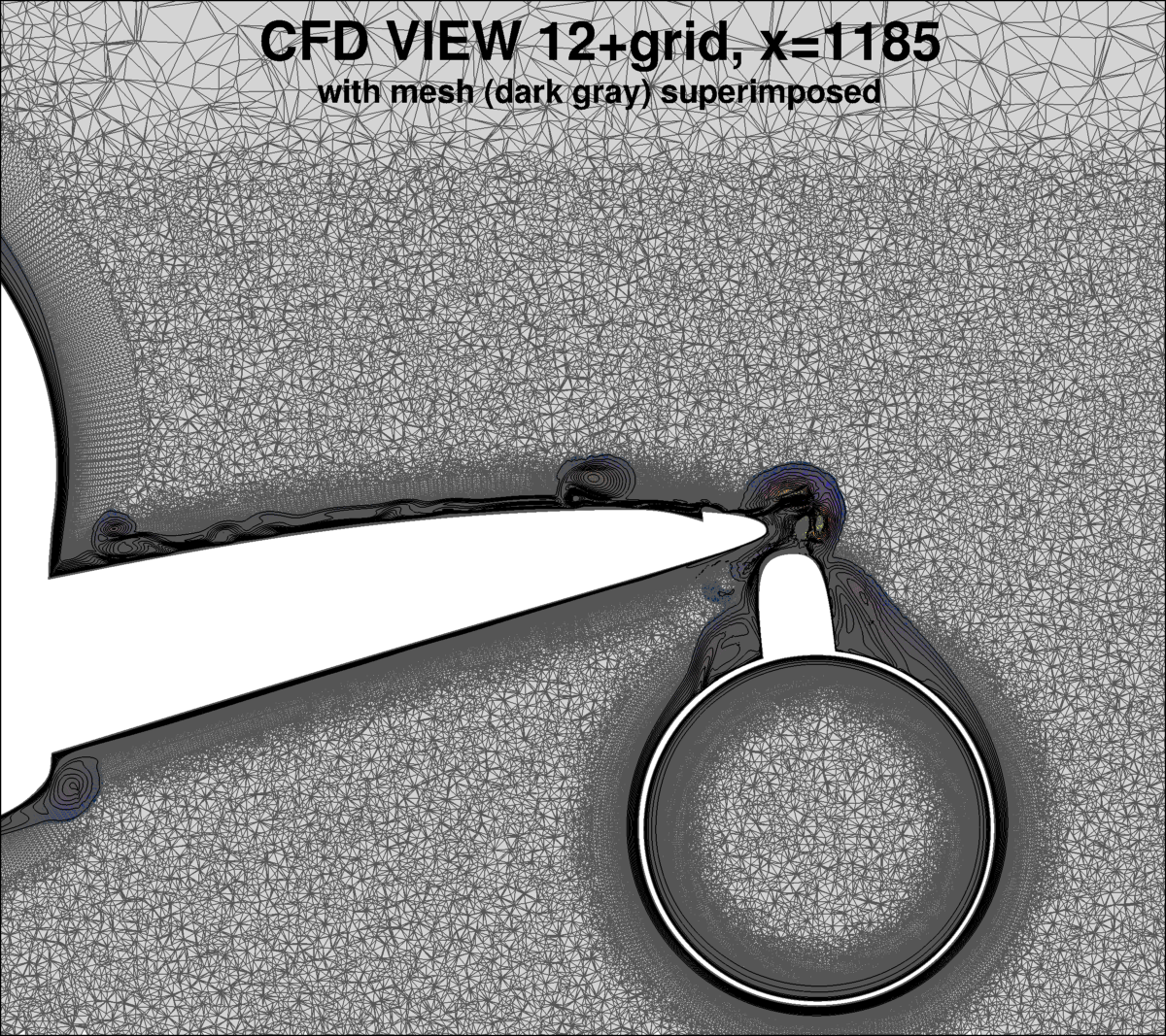
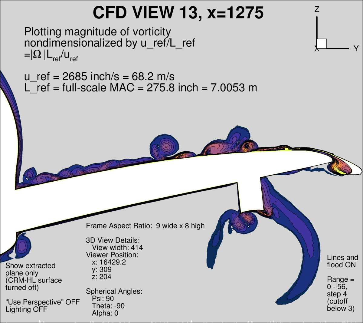
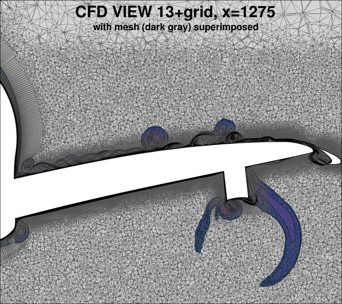
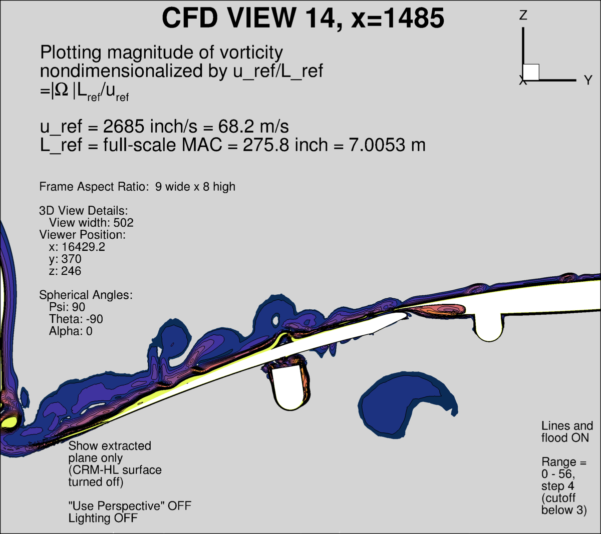
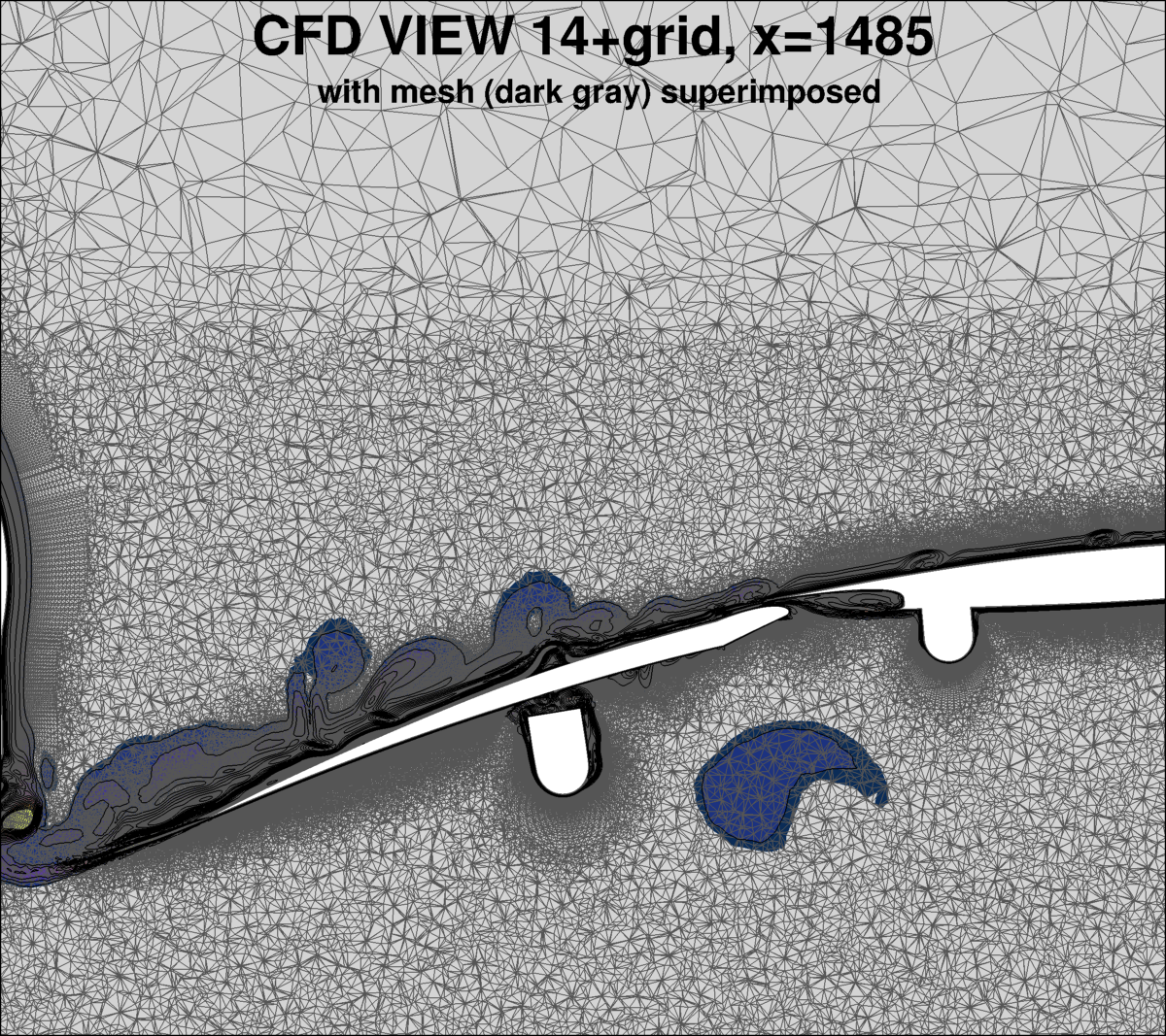
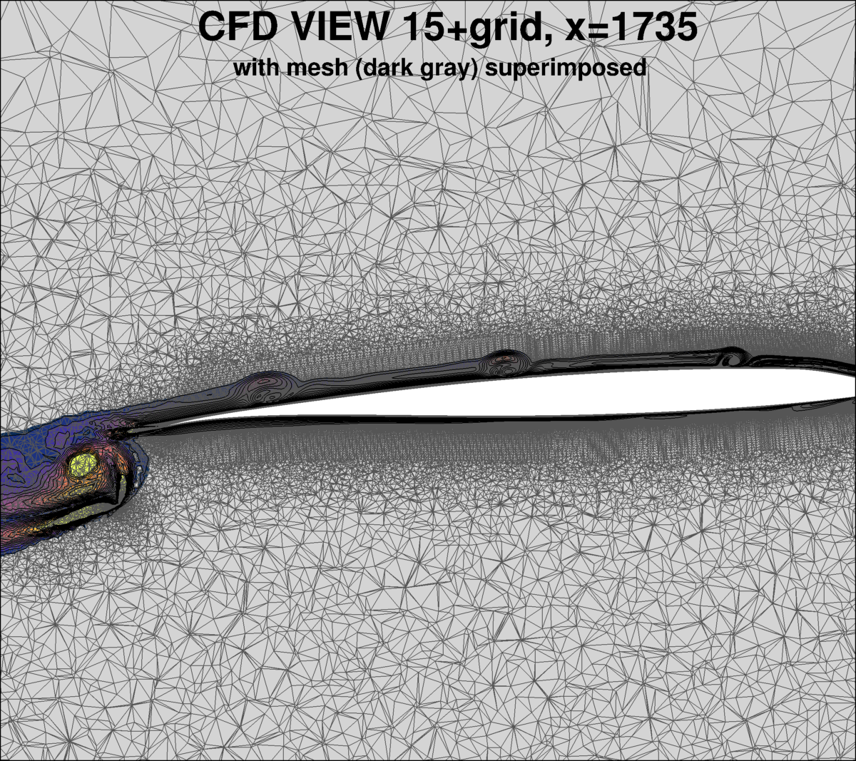
The 5 desired views are shown below (two plots for each view, with and without some appropriate representation of the mesh superimposed).
Each view is looking directly forward, with only the extracted plane shown. The
body surface is not included on any plot. The view details are provided on the plots below. These plots use
Tecplot's "cmocean - thermal" color map (banded), which is a thirteen point color spectrum from blue to cyan to green to yellow to red
(see vortmap_tecplot.map, renamed here, but it is identical to Tecplot's cmocean - thermal).
It is given by:
| LEVEL
|
R
|
G
|
B
|
| 0.00
|
3
|
35
|
51
|
| 0.1
|
15
|
49
|
105
|
| 0.15
|
35
|
51
|
140
|
| 0.2
|
63
|
51
|
159
|
| 0.3
|
103
|
67
|
150
|
| 0.4
|
138
|
82
|
140
|
| 0.5
|
176
|
95
|
129
|
| 0.6
|
213
|
107
|
108
|
| 0.7
|
242
|
130
|
76
|
| 0.8
|
251
|
165
|
60
|
| 0.85
|
250
|
186
|
62
|
| 0.9
|
246
|
208
|
69
|
| 1.00
|
231
|
250
|
90
|
and the recommended range (shown in the figure) is 0 to 56, step 4 (banded), with cutoff below 3.
If your method is unsteady, then vorticity contours based on mean velocity should be plotted.


The Tecplot layout files for the above five views are provided here:
XXX_cfdview_11_x1095_thermal.lay,
XXX_cfdview_12_x1185_thermal.lay,
XXX_cfdview_13_x1275_thermal.lay,
XXX_cfdview_14_x1485_thermal.lay,
XXX_cfdview_15_x1735_thermal.lay.
Note that these files are most likely NOT directly applicable to most participants' data (in particular they assume that the
variable "vort_mag" is already appropriately nondimensionalized); therefore
they should be used for guidance only.
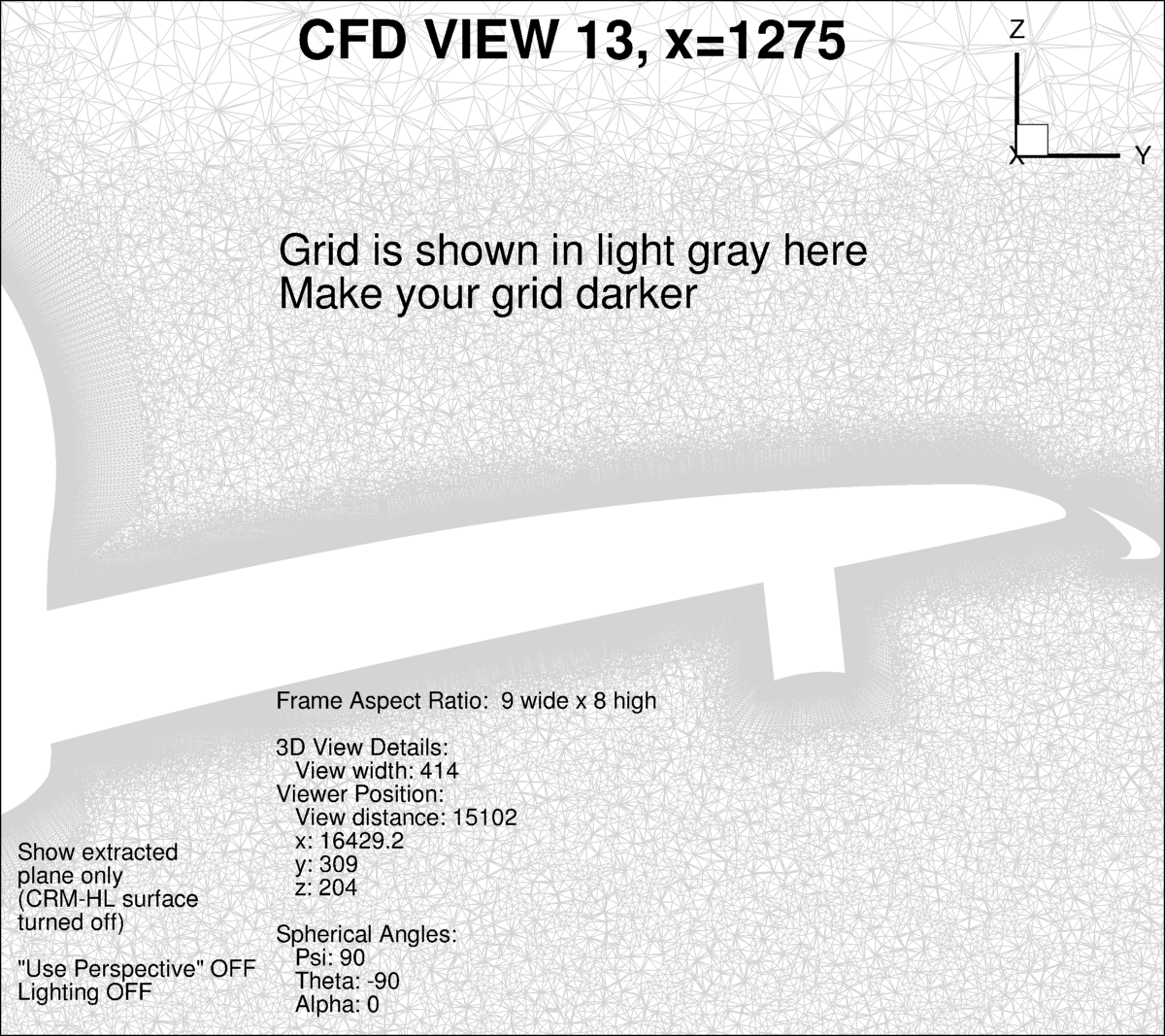
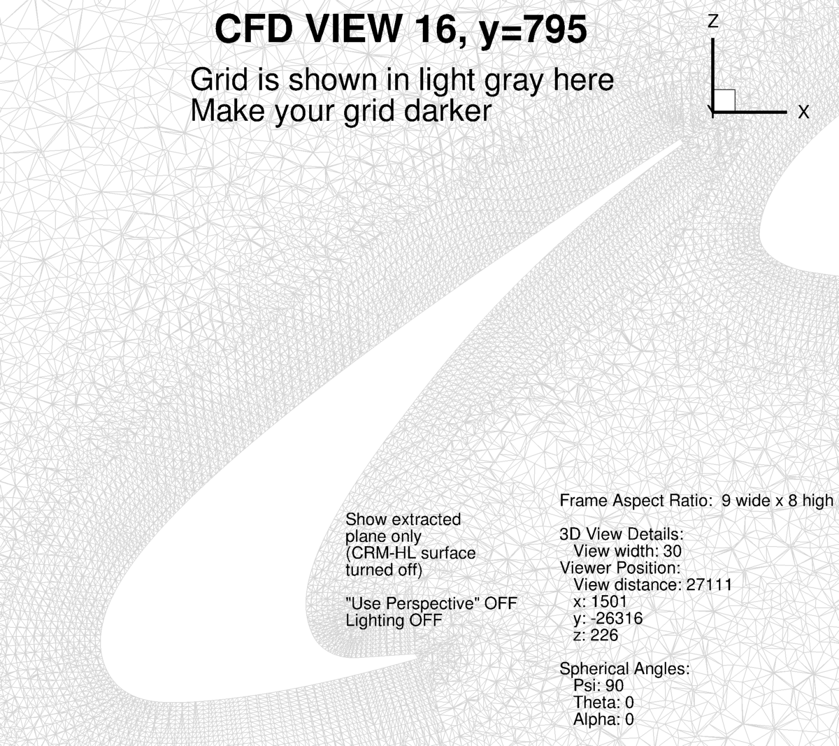
Some views are considered useful for picturing CFD grid characteristics in particular planes.
Below are two such views. One is the same as CFD VIEW 13 (above), while the other is a new y=const plane.
The Tecplot layout files for the above two views are provided here:
XXX_cfdview_13_x1275_gridonly.lay,
XXX_cfdview_16_y795_gridonly.lay.
Note that all of the above assumes that your grid is in full-scale inches! If your grid is in different
units, please be sure to translate to full-scale inches prior to submittal. For example, if your grid
is in full-scale meters, then (if you are using Tecplot) execute:
- {x}={x}*39.37
- {y}={y}*39.37
- {z}={z}*39.37
to translate it to full-scale inches prior to proceeding. The above Tecplot macros should then work,
and the CFD views should be relevant.
One of the participants (Andrew Lofthouse) has kindly provided some Tecplot scripts that have helped him to plot
the streamline and skin friction CFD views and vorticity plots. There is no guarantee they will work
for you, but feel free to try them:
Return to: High Lift Prediction Workshop Home Page
Recent Significant Site Updates
06/13/2024 - Added Tecplot layout files for grid-only views 13 and 16
05/24/2024 - Added 1-page templates for participants to record a summary of their method
04/30/2024 - Added grid-only views: CFD VIEW 13 and 16
04/10/2024 - Updated data submittal form to v10
01/18/2024 - Updated data submittal form to v9; also added Lofthouse's Tecplot scripts
11/09/2023 - Updated data submittal form to v8
11/03/2023 - Updated data submittal form to v7
10/06/2023 - Added explanation regarding Case 2's Row C surface extraction
09/23/2023 - Updated the Tecplot surface pressure and skin friction cutters, now somewhat different for each test case
08/17/2023 - Added CFD View SP2.1 and SP2.2, specifically for Case 2, to focus on horizontal tail
08/03/2023 - Updated data submittal form to v6
06/12/2023 - Minor update to Case 1 data submittal form (in participant info file only)
06/08/2023 - Added CFD View SP1.1, specifically for Case 1, to focus on outboard wing trailing edge
05/05/2023 - Posted Case 1 data submittal form XXX_Case1_Lastname_Code_Model_v2.tar.gz
Privacy Act Statement
Accessibility Statement
Responsible NASA Official:
Li Wang
Page Curator:
Li Wang
Last Updated: 08/13/2024
